In [0]:
import pandas as pd
import numpy as np
import matplotlib.pyplot as plt
import math
In [63]:
raw_data = {'x1': [0.15, -0.1, 0, -0.25, 0.05],
'x2': [3500, 3400, 4000, 3900, 3200],
'y': [8, 5, 3, 1, 7]}
df = pd.DataFrame(raw_data)
df
Out[63]:
In [64]:
plt.figure(figsize=(10, 7))
plt.scatter(df.x1,df.x2, label="Without scaling", color='blue')

plt.grid(True, alpha=0.6)
plt.title("Scatter", fontsize=20)
plt.xlabel("x1", fontsize=20)
plt.ylabel("x2", fontsize=20)
plt.legend()
plt.show()

In [0]:
def stddev(c):
    v = 0
    mn = round(sum(c),2)/len(c)
    for i in range(len(c)):
        v += (c[i]-mn)**2
    v /= len(c)
    return math.sqrt(v)
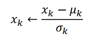
1.a) Scaling by normalization
In [0]:
def scalingByNormalization(c):
  newc = [None] * len(c)
  mean = round(sum(c),2)/len(c)
  sdev = stddev(c)
  for i in range(len(c)):
    newc[i] = (c[i] - mean)/ sdev

  return newc
In [0]:
nx1= scalingByNormalization(df.x1)
nx2= scalingByNormalization(df.x2)
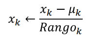
1.b) Scaling by range
In [0]:
def scalingByRange(c):
  newc = [None] * len(c)
  mean = round(sum(c),2)/len(c)
  r = max(c)- min(c)
  for i in range(len(c)):
    newc[i] = (c[i] - mean)/ r

  return newc
In [0]:
mx1= scalingByRange(df.x1)
mx2= scalingByRange(df.x2)
In [70]:
plt.figure(figsize=(10, 7))
plt.scatter( nx1, nx2 ,label="Feature scaling by Normalization", color='orange')
plt.scatter(mx1, mx2 ,label="Feature scaling by range", color='green')


plt.grid(True, alpha=0.6)
plt.title("Scatter", fontsize=20)
plt.xlabel("x1", fontsize=20)
plt.ylabel("x2", fontsize=20)
plt.legend()
plt.show()

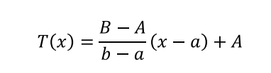
1.c) Scaling between range
In [0]:
def scalingBetweenRange(c, r1, r2):
  newc = [None] * len(c)

  for i in range(len(c)):
    newc[i] = ((r2-r1)* ((c[i] - min(c))/(max(c)-min(c)))) + r1

  return newc
In [0]:
ny= scalingBetweenRange(df.y,-10, 20)
In [73]:
df2 = pd.DataFrame(list(zip(nx1, nx2, mx1, mx2, ny)),
               columns =['x1N', 'x2N', 'x1R', 'x2R', 'ny'])
df2
Out[73]:
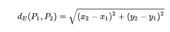
2.a) Euclidean distance
In [0]:
def euclidian(c1, c2):
	d=0
	for i in range(len(c1)):
		d += math.pow(c2[i] - c1[i], 2)
	return math.sqrt(d)
In [75]:
v1 = [2, 1]
v2 = [3, 4]
print(euclidian(v1, v2))
2.b) Manhattan distance
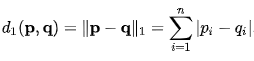
In [0]:
def manhattan(c1, c2):
	d=0
	for i in range(len(c1)):
		d += abs(c1[i] - c2[i])
	return d
In [77]:
v1 = [2, 3]
v2 = [1, 4]
print(manhattan(v1,v2))
2.c) Chebyshev distance

In [0]:
def Chebyshev(c1, c2):
  subtractions = [None] * len(c1)
  for i in range(len(c1)):
    subtractions[i] = abs(c2[i] - c1[i])

  return max(subtractions)
In [79]:
v1 = [2, 1]
v2 = [3, 4]
print(Chebyshev(v1, v2))
2.d) Minkowski distance
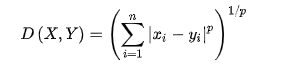
In [0]:
def Minkowski(c1,c2, p):
  pp = 1/p
  d=0
  for i in range(len(c1)):
    d +=  math.pow(abs(c1[i] - c2[i]),p)

  return math.pow(d, pp)
In [81]:
v1 = [2, 1]
v2 = [3, 4]
print(Minkowski(v1,v2,0.7))
3. Suppose you want to apply the multiple linear regression method to a database whose variables or factors are shown in the image below. Let's also assume that at the moment only the following variables will be used to build the model:
- ### Independent variables: season, hour, workingday, windspeed
- ### Dependent variable: registered
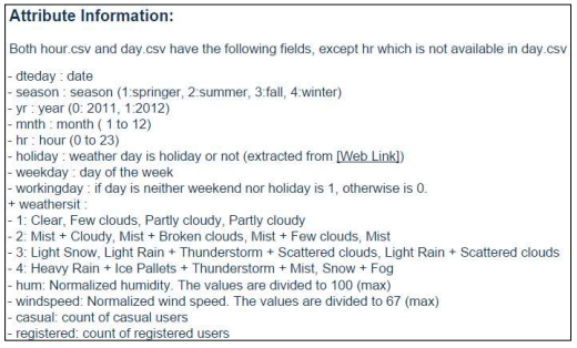
3.a) Indicate what type of variable each one is: categorical or numerical. If it is numerical, so indicates whether it is discrete or continuous.
- Categorical: Season, workingday
- Numerical: registered(discrete), hour(discrete), windspeed(continuous)
3.b) In the case of categorical variables, indicate the dummies variables that you believe should be introduced to the model, indicating the base case of each of these dummy variables, or if you decided not to use base case and instead add a additional dummy variable. The base case is the variable that is considered in the model when all other dummy variables in that case are zero.
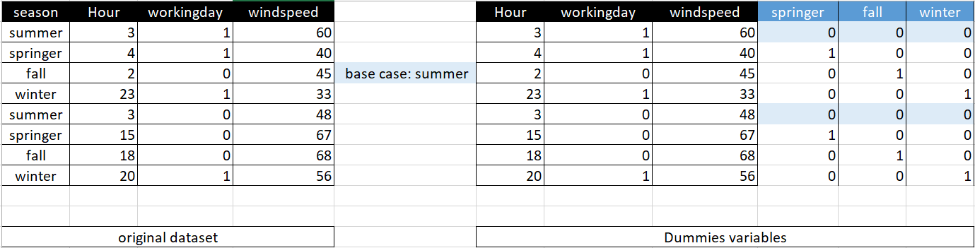
3.c) How many dummy variables were added? It indicates how the symbolic representation of the multiple linear regression model would look like when all independent, dummy or non-dummy variables are included.
- ### y= Bo + B1hour + B2workingday + B3windspeed + D1springer + D2fall + D3winter + E