A New Approach for Efficient Sequential Decoding of Static Huffman Codes
The exponential growth of the volume of data, the high cost of storage and high latency create robust lines of research in the area of data compression, compression speed is a transparent process for the end user since the data compression process are currently running and hosted in the cloud, but the decompression process impacts directly on the quality of service (QoS) offered to the end user and this makes the decompression process an area of study of equal importance. Therefore, the static huffman algorithm can be measured in two ways, one in terms of how the storage space is reduced and the other in terms of decoding speed. This research proposes an approach to decoding static Huffman codes based on the amount of information accumulated in the code lengths assigned to symbols of a dataset by the static huffman algorithm, the ascending order of the Huffman table based on the length code is not the best sequential decoding option for heterogeneous datasets, this study quantified the results related to the decompression speed and significant results were achieved, it also uses methodology that helped in the observation of the entire pipeline of compression and decompression.
Problem Statement
Companies in all sectors need to find new ways to control the rapid growth of the volume of their heterogeneous data generated every day, for this reason mentioning Velocity, Volume and Variety (Laney, 2001) are key concepts to strengthen this document.

Velocity
data must be stored, extracted, transmitted and converted into information quickly before it loses its value. Studies on compression and decompression algorithms could directly impact the speed of how this data is transmitted in real time and could also improve latency in distributed systems.
Volume
Currently, the main providers of cloud services such as Amazon Web Services (AWS), Microsoft Azure, Google Cloud and IBM OpenWhisk (Expósito and Zeiner, 2018), are responsible for storing all types of files in their Data Centers, generating an immense amount of daily information (which in some cases reaches petabytes), which has a high cost associated with the storage and maintenance of data.
Variety
The data is highly heterogeneous, this implies that it can be generated by spacecraft, radio telescopes, telescopes, medical images, social networks, sensors, banking transactions, flight data, smartphones, cameras, GPS and DNA sequences, among others. It can be structured and unstructured data, but in the end it is stored on a server as a string of bits, therefore, focusing on designing, observing and improving a scheme in the decoding of static huffman codes process that is optimal and supports any type of data is essential.
Proposed methodology
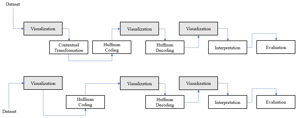
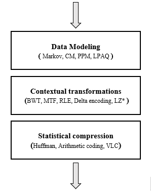
As this research is based on the study of the decoding of static Huffman codes and measuring its performance in a sequential environment, it is necessary to get directly involved with the coding using the Huffman algorithm, for this reason, it is necessary to generate the huffman codes using different datasets. Huffman is not dedicated to compress text only, because Huffman always expects a sensitive and transformed dataset for reach a good rate compression, in a business environment the compression pipeline use contextual tranformations in previous stages before applying a statistical compression, these transformations aim to lower the entropy of the entire dataset and make it sensitive to reach best rate compressions. The proposed methodology turns out to be adequate to choose the best decoding algortihm, the phases were explained above.
Contextual transformations
Modern compression tools and techniques are not based solely on the use of a compression algorithm, actually the use of this is part of the final stage of an entire compression pipeline, but before reaching the last one, there is a stage called contextual transformations that are responsible for reorganizing the symbols of the data set so that they are more sensitive to statistical compression methods such as Huffman, in other words they are artificial generators of redundancy, two of the main algorithms that will be explained in this research are the BWT and the MTF.
It should be noted that the Huffman algorithm is widely used in many known compression tools or codecs, the image below shows the compression pipelines of some of these tools and we can see that the huffman coding is very common in much of them
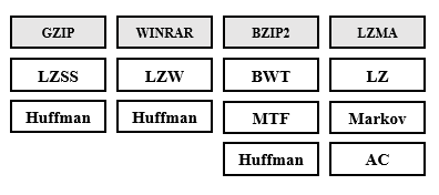
On the other hand, it is relevant to mention that Hadoop is one of the most famous tools to control and manage large amounts of data and is composed of the most robust codecs for compressing its formats, The blocks in bzip2 can be independently decompressed, bzip2 files can be decompressed in parallel, making it a good format for use in big data solutions with distribuited computing frameworks like Hadoop, Apache Spark, and Hive

Static Huffman coding
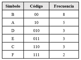
One of the algorithms most used by different current data compression tools and which is part of the final stage of the entire compression pipeline is the Huffman algorithm, due to its nature of optimizing the construction of variable length codes, or In other words, the average length of the generated codes is very close to the minimum expected according to entropy formula, this algorithm was created by David Huffman in 1952 and since its creation to the present it has been a topic of relevant and very important research in the area of data compression, the algorithm achieves its best performance when the probabilities of the symbols are negative powers of 2, the steps taken by the algorithm to generate variable length codes are described below , we will use the next dataset.
ABCDBEFBAABCDBEABCDBEFBA
The frequency of occurrence of each symbol is calculated and ordered in a leaf node type data structure, which later will form part of a binary tree.

The two leaf nodes with the smallest probabilities are taken and a parent node is created that has the sum of the probabilities of each selected leaf node
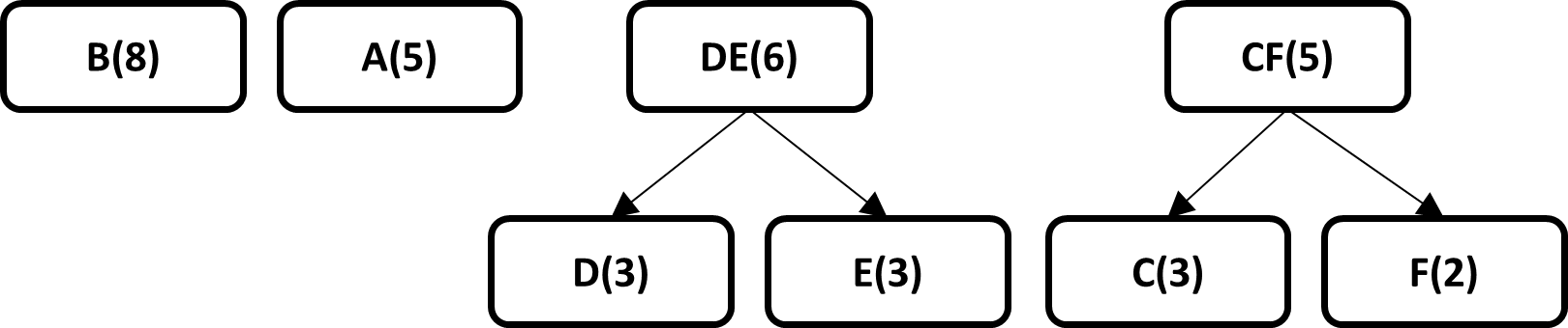
The same process is followed always taking into account the following smallest probabilities of leaf nodes, parent nodes or leaf nodes and parents.
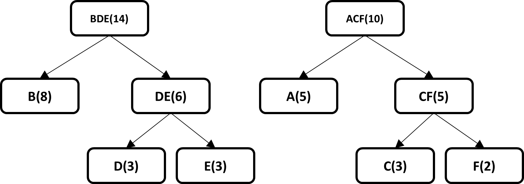
The end result is a binary tree where the leaves of the tree have the original probability of each symbol, the code for each symbol is generated by traversing the tree from the root node to each leaf.
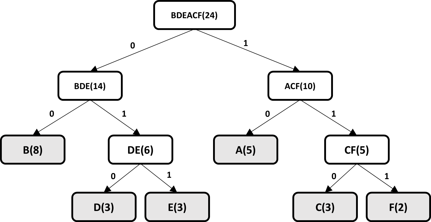
Taking into account that there are 6 different symbols contained in the original data set, the best way to represent each symbol is with 3 bits, since 6 is in 2^3, therefore, the original data set has 72 bits , the Huffman algorithm achieves a compressed string with a length of 59 bits
Huffman decoding
The Huffman code decoding process seems to be somewhat trivial, but it is not, until today studies with different points of view and approaches continue to be thrown to try to improve response times in the decoding process, due to that the decompression time of the data directly impacts the user experience and the compression time will always be transparent for the user, the importance is very clear. The classical sequential decoding techniques are also used internally in the techniques based on parallelism or techniques that make better use of hardware resources, therefore, an advance in sequential decoding also involves an advance in the parallel decoding of Huffman codes, below , the basic sequential decompression techniques that are commonly used in the modern data compression and decompression pipeline will be explained
Standard Decoding of Variable Length Codes
This technique is based on the use of a Lookup-Table to find the pattern that matches some code in the Huffman table, the technique manages to decode the pattern of compressed bits, but it is slow, and the number of attempts for each symbol is expressed by the first equation, where F means attempts per symbol or number of failures, which means that the algorithm fails to decode each symbol L - 1 times, where L represents the length of the code for the symbol, the global number of failures for decoding all the symbols in the original data set is expressed by the second equation, where Fr is the frequency of each different symbol
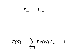
For the previous data set, decoding the 24 symbols of the compressed bitstream pattern has a cost of 35 attempts, although the symbols involved in the second equation are the different symbols that appear in the Huffman table, in this case they are 6 different symbols, the objective of measuring the failure is to find a relationship that leads us to reduce it to try to improve the overall response time of the algorithm.
ABCDBEFBA.....
1000110010000111110010
10(A)00(B)110(C)010(D)00(B)011(E)111(F)00(B)10(A)</br>
  class lookup_decoding:

    def __init__(self, cf, ht):
        self.cf = cf
        self.ht = ht

    def decode(self):
        o_file = []
        c_size = len(self.cf)
        buffer = []

        for i in range(0, c_size):
            buffer.append(self.cf[i])
            possible_code = ''.join(buffer)
            if possible_code in self.ht.keys():
                o_file.append(self.ht[possible_code])
                buffer.clear()

        return o_file
Decoding based on Code Length
Another approach to sequential decoding is to take into account the lengths of the code as a fixed general reference pattern that helps us reduce the number of attempts, the huffman table was modified with the lengths of each code and is shown below
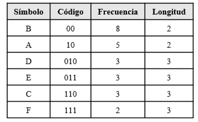
The central idea of this approach is to make cuts on the compressed bit string of size m, where m is an element that belongs to the set Lm, and Lm is the set of all the lengths found, for the previous case the set Lm is { 2, 3}, and its cardinality is 2, we will call the cardinality | Lm |, therefore, in the worst case, decoding each symbol involves trying | Lm | - 1 times, in order to achieve the best performance of this technique, the code lengths must be ordered from smallest to largest, because shorter length codes have a higher probability of occurrence, ascending order will definitely reduce the number of attempts response time in decompression.
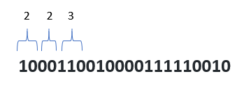
ABCDBEFBA.....
1000110010000111110010
10(A)00(B)110(C)010(D)00(B)011(E)111(F)00(B)10(A)</br>
class length_code_decoding:

    def __init__(self, cf, ht, lc):
        self.cf = cf
        self.ht = ht
        self.lc = lc

    def decode(self):
        o_file = []
        c_size = len(self.cf)

        index = 0
        while index < c_size:
            for sz in self.lc:
                possible_code = self.cf[index: index + sz]
                if possible_code in self.ht.keys():
                    o_file.append(int(self.ht[possible_code]))
                    index = index + sz
                    break

        return o_file
Decoding based on Huffman Tree Reconstruction
This decompression technique is not recommended, because the tree traversal is bit by bit, the number of instructions that are executed end up giving the same results of the first approach, in addition to this, the construction of the tree from the table Huffman creates another unnecessary cost by affecting decompression times.
Decoding with Markov Chains
The different lengths of the generated codes can be seen as a sequence of events that follow a stochastic process, there are always different lengths of codes, which can represent the states, each length is associated with a probability, and there is memory loss, the reading a future code length only depends on the previous reading. Due to these very clear properties, decompression based on a Markov chain does not sound out of place, and it is a lossless decompression approach, however, using a Markov chain demands storage to store the transitions matrix and this puts the compression rate achieved at risk.
class MarkovChain(object):

    def __init__(self, transition_matrix, states):
        self.transition_matrix = np.atleast_2d(transition_matrix)
        self.states = states
        self.index_dict = {self.states[index]: index for index in
                           range(len(self.states))}

        self.state_dict = {index: self.states[index] for index in
                           range(len(self.states))}

    def fix_p(self, p):
        if p.sum() != 1.0:
            p = p*(1./p.sum())
        return p

    def next_state(self, current_state):
        return np.random.choice(
         self.states,
         p=self.fix_p(self.transition_matrix[self.index_dict[current_state], :])
        )


    def generate_states(self, current_state, no=10):
        future_states = []
        for i in range(no):
            next_state = self.next_state(current_state)
            future_states.append(next_state)
            current_state = next_state
        return future_states

class MKC_decoding:

    def __init__(self, cf, ht, lc, mtx):
        self.cf = cf
        self.ht = ht
        self.lc = lc
        self.mtx = mtx

    def decode(self):
        o_file = []
        f_list = []
        s_list = []
        c_size = len(self.cf)

        predict_length = MarkovChain(transition_matrix=self.mtx , states=self.lc)

        next_state_length = 0
        for sz in self.lc:
            possible_code = self.cf[0: sz]
            if possible_code in self.ht.keys():
                o_file.append(self.ht[possible_code])
                next_state_length= sz
                break

        index = next_state_length
        while index < c_size:
                next_state_length = predict_length.next_state(current_state=next_state_length)
                possible_code = self.cf[index: index + next_state_length]
                if possible_code in self.ht.keys():
                        o_file.append(self.ht[possible_code])
                        index += next_state_length

        return o_file
Results
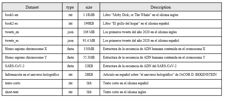
Choosed datasets
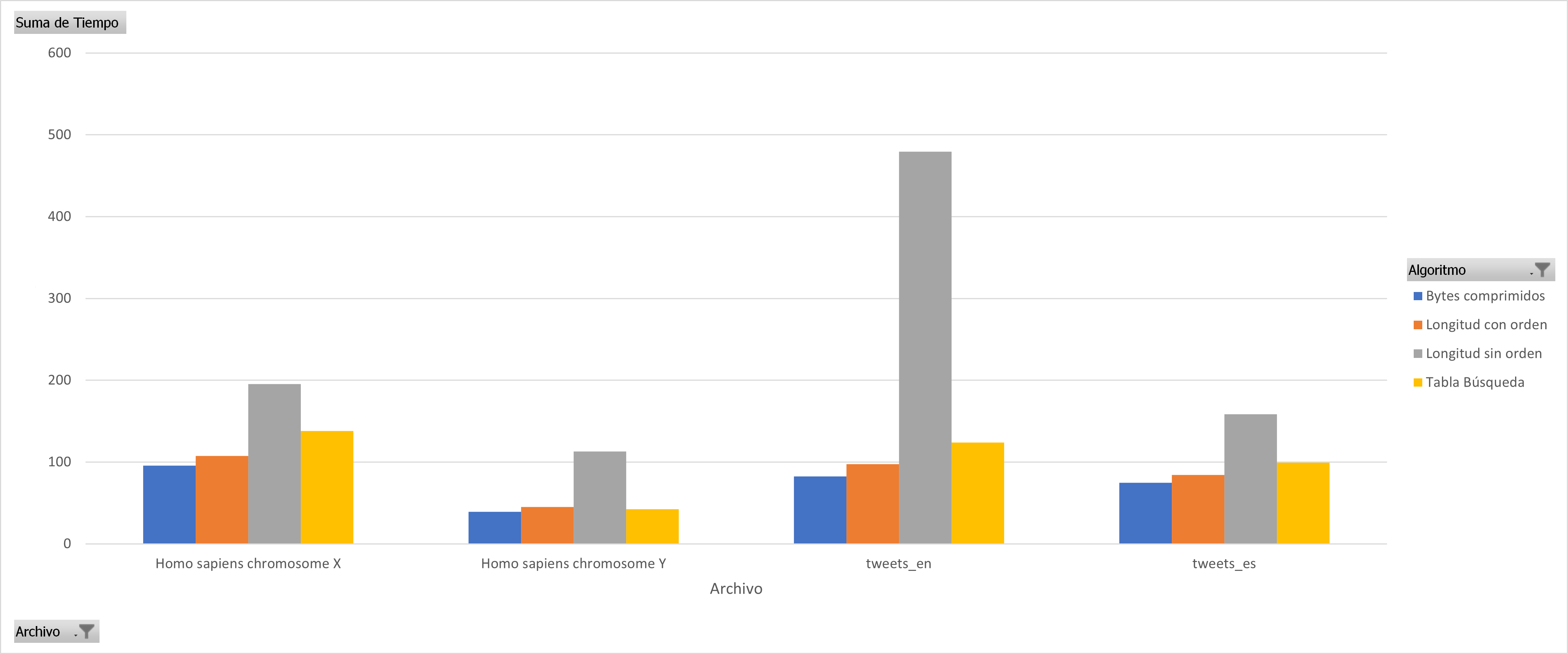
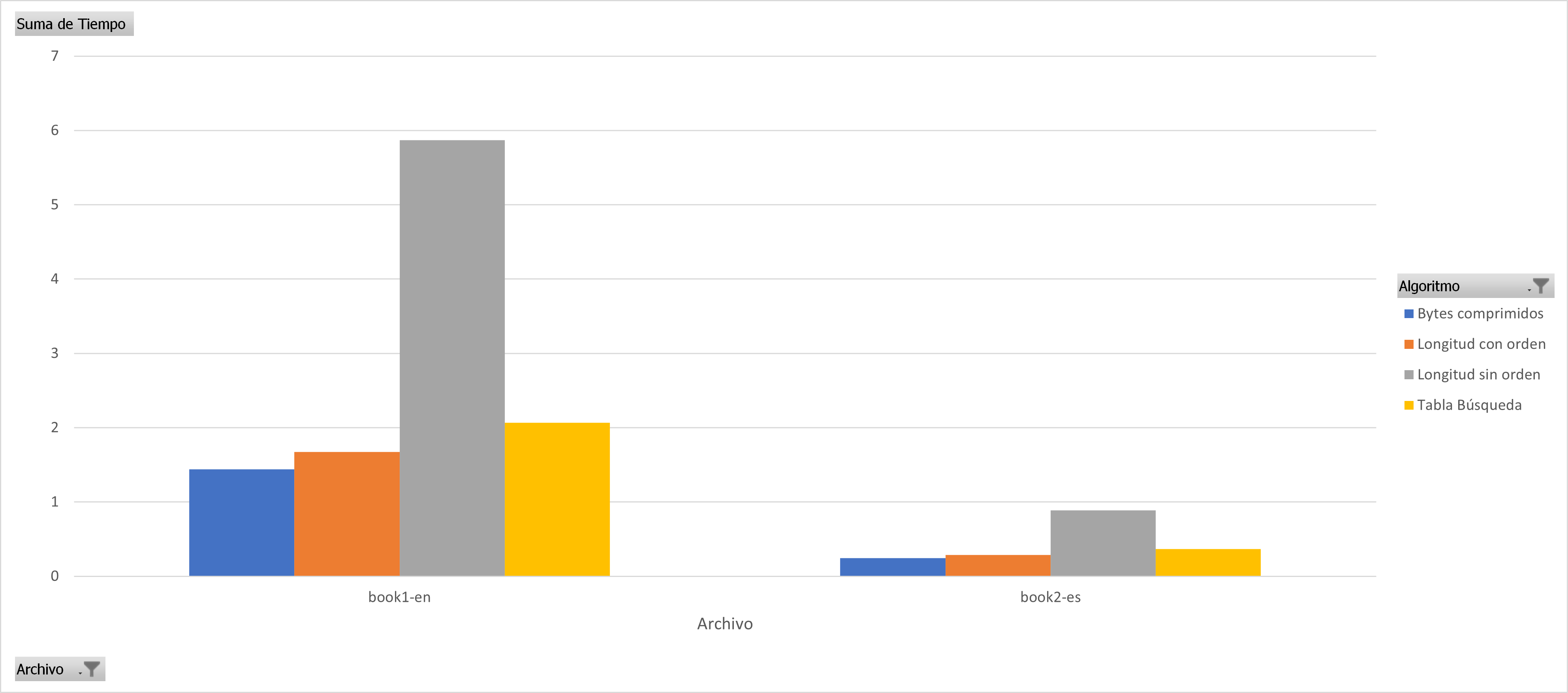
Based on the proposed methodology, we will use the following datasets to be able to see the behavior in compression and then in decompression of each dataset.
Visualization of the symbols distribution
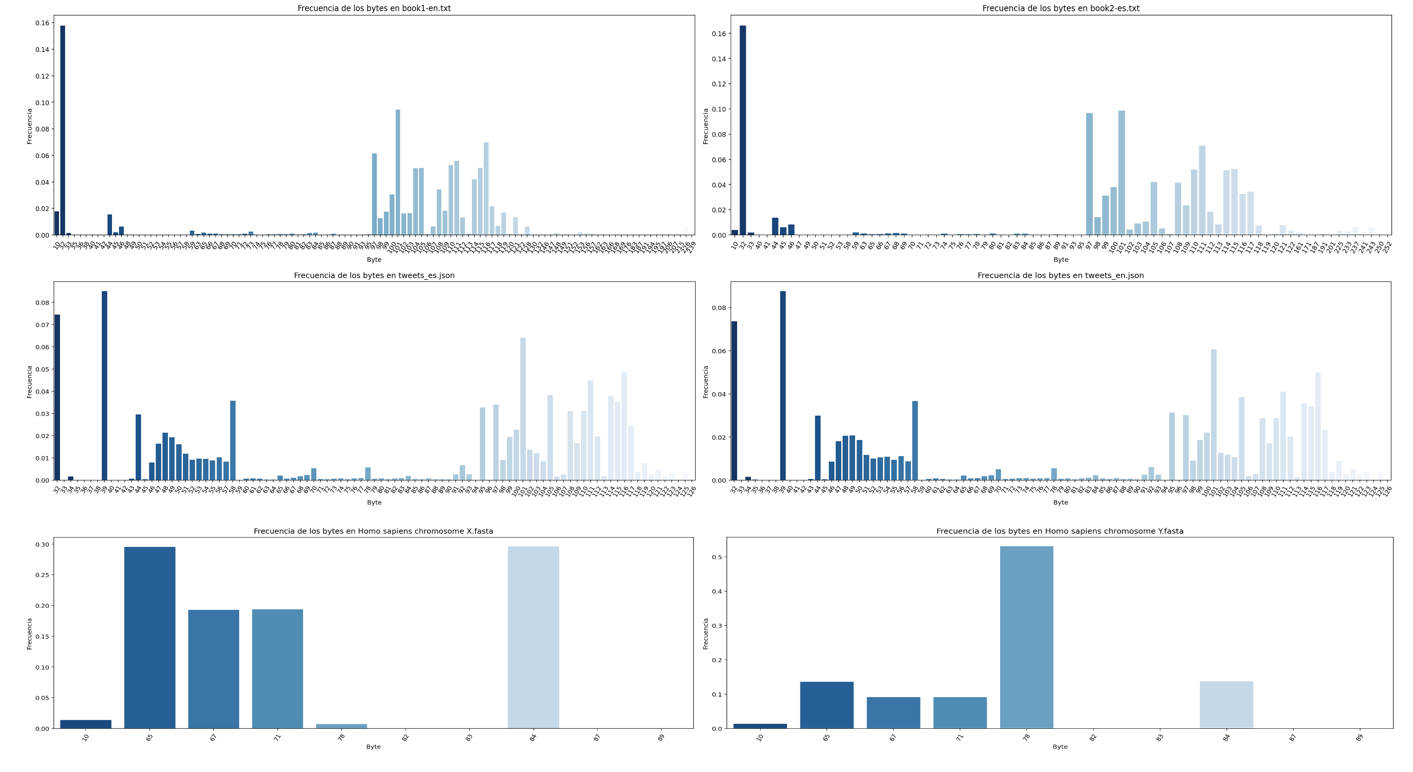
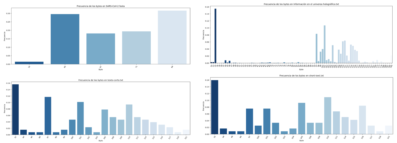
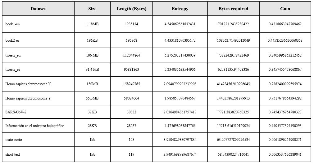
The Graphs with the distribution of symbols of each file are shown below. In most cases and because the content of some files is in natural language, Benford's law can be observed, there is a large amount of information accumulated in bytes that begin with the number 1, it can also be observed that there is a large amount of information accumulated in three-digit bytes, for .fasta files it can be observed the presence of a very short alphabet and special symbols that are related to the structure file standard, the last table in this section shows a numerical summary of the entropy analysis of each file, the necessary bytes and gain columns are related to the following formulas consecutively

Contextual transformations
In this phase, what is intended is to transform the symbols of the data sets to a new set of symbols with lower entropy, the decline of this gives us a signal of the gain in storage and possibly a lower compression rate, consequently a process faster decompression, as already mentioned above we will first use the BWT algorithm and its output will be the input of the MTF algorithm, the final output of the last one mentioned will be used to measure the entropy in each file and in this way demonstrate the benefit of a transformation contextual, the table shows the new entropies for each data set, it can be observed that the entropy value slightly decreases and the gain value rises, there is an additional column called "BWT (Window Size)" this column indicates the size of the piece in bytes that the BWT algorithm handled, the Graph shows the new gain in orange and in almost all cases using BWT favors compression, At the last graph we can now select the files that BWT and MTF will use and those that will not.

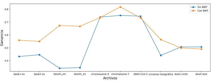
The files that will use the BWT and MTF in the compression pipeline are book1-en, book2-es, tweets_en, tweets_es, Homo sapiens chromosome Y and Information in the holographic universe, because they are the ones that present a significant gain.
Data compression with static Huffman
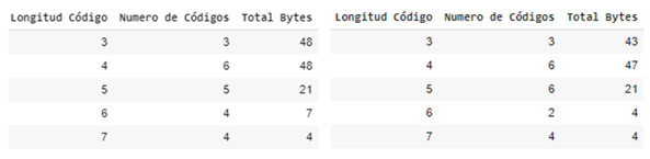
Once the decision of which datasets will go through a contextual transformation has been made, the statistical compression is carried out with the static Huffman algorithm, the table shows the compression factors achieved, a high compression rate is better, you can also Note that the compression percentage achieved is close to the gain calculation of the previous tables, this section concentrates more on the observation of the generated Huffman code lengths, therefore we also show the result of these lengths with the amount of Huffman codes. that length and the amount of bytes that the length has accumulated, it will not be necessary to show the code generated by each symbol and its associated frequency, we are assuming that Huffman optimized the variable code length as much as possible based on the entropy calculation of the data set.

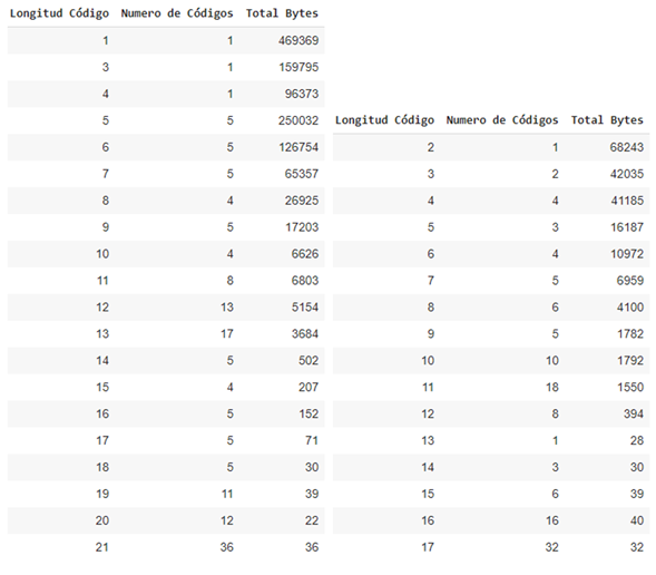
Summary tables of generated code lengths for the book1-en.txt and book2-es.txt data sets from left to right
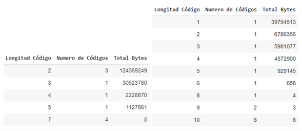
Summary tables of generated code lengths for the texto-corto.txt and short-text.txt data sets from left to right
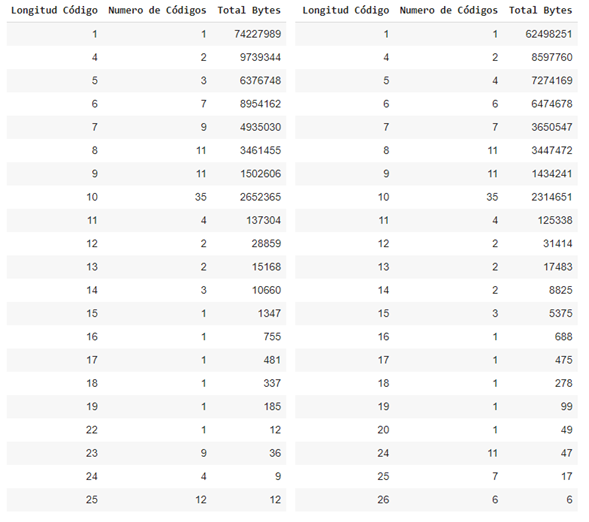
Summary tables of generated code lengths for the Homo sapiens chromosome X.fasta and Homo sapiens chromosome Y.fasta data sets from left to right

Summary tables of generated code lengths for the SARS-CoV-2.fasta e Información and el universo holográfico.txt data sets from left to right
Summary tables of generated code lengths for the tweets_en.json and tweets_es.json data sets from left to right
It can be seen in the previous tables that the code lengths are sorted in ascending order, this in order to improve the decoding process using chunks of the compressed chain of the shortest possible length and speed up response times due to the fact that the symbols encoded with a shorter code length are more likely to occur.
Visualization of the code lengths distribution by symbols
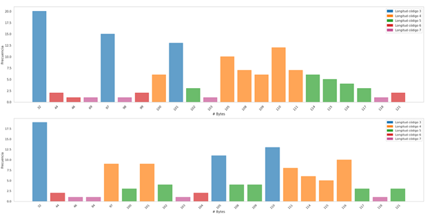
Below, the distribution of the code lengths per symbol for each dataset is shown, there are common features that are independent of the probability distribution of the symbols, we can see that for datasets that have information in natural language, most of the information is concentrated in symbols or bytes of length 3, another relevant feature that is common in uniform and non-uniform distributions is the presence of Benford's law, there are more symbols that begin with the number 1, the objective of this phase is to visualize that Symbol groups contain more information and what length of code is associated with them.

Distribution of code lengths by symbols for the book1-en.txt and book2-en.txt datasets

Distribution of code lengths by symbols for the tweets_en.json and tweets_es.json datasets

Distribution of code lengths by symbols for the Homo sapiens chromosome X.fasta and Homo sapiens chromosome Y.fasta datasets

Distribution of code lengths by symbols for the SARS-CoV-2.fasta and Información en el universo holográfico.txt datasets
Distribution of code lengths by symbols for the texto-corto.txt and short-text.txt datasets
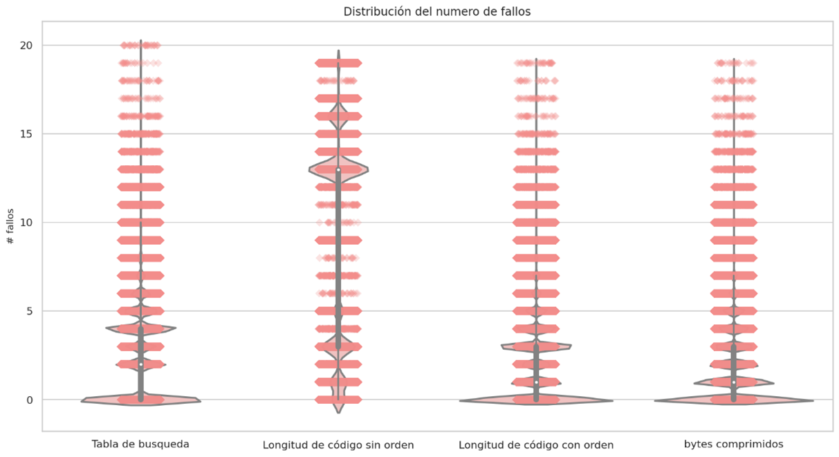
Huffman Decoding and visualization
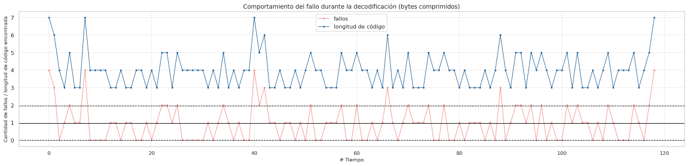
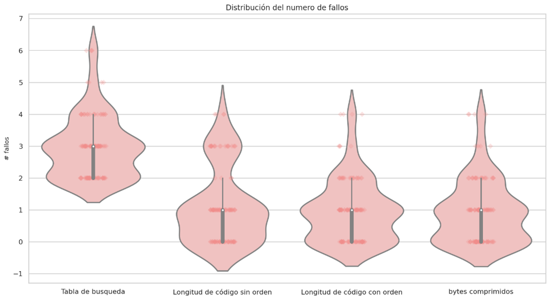
Due to the observations in the previous section, it is notable that there are lengths of codes that are not the shortest that contain more compressed information, it is for this reason that a new approach is proposed to order the huffman table based on the amount of compressed information descending and not ascending by code lengths, the final results are discussed later. The decompression behavior will only be shown for some relevant datasets where the improvement is meaningful.
book1-en.txt

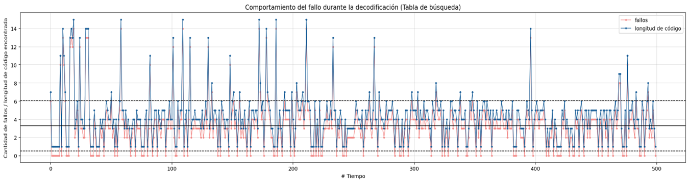
Failure behavior during decoding using a lookup table

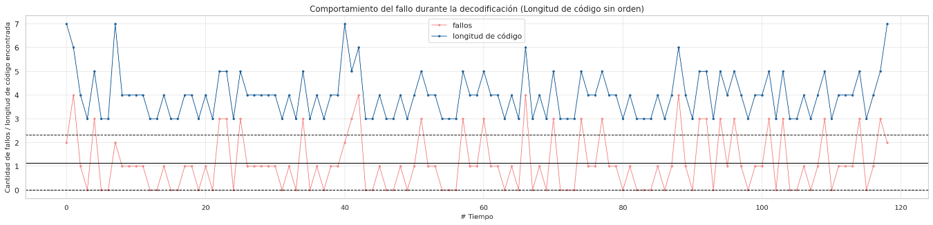
Failure behavior during decoding without sorted

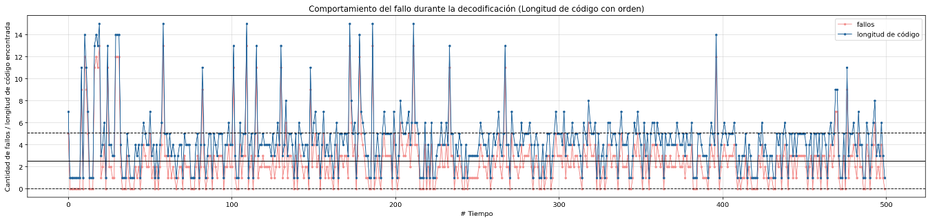
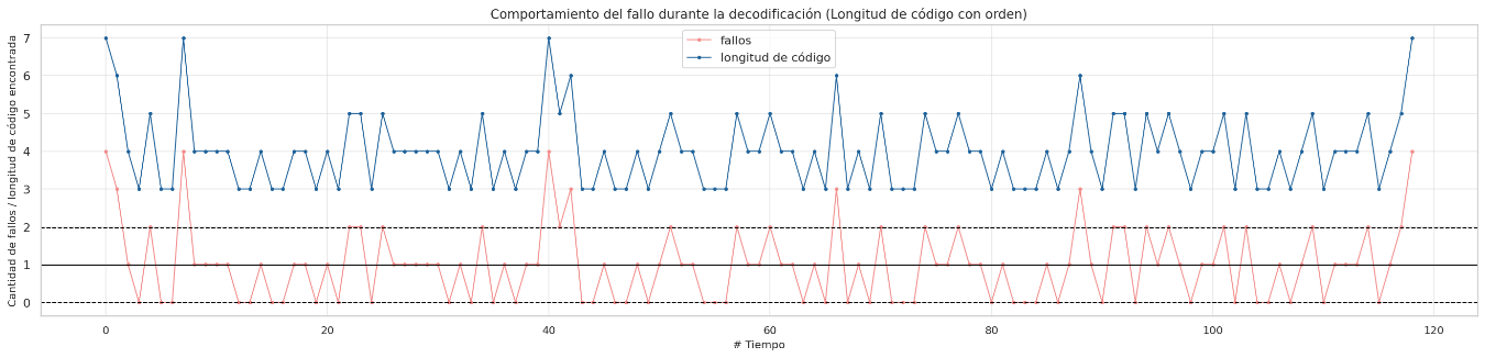
Failure behavior during decoding sorted by lenght codes
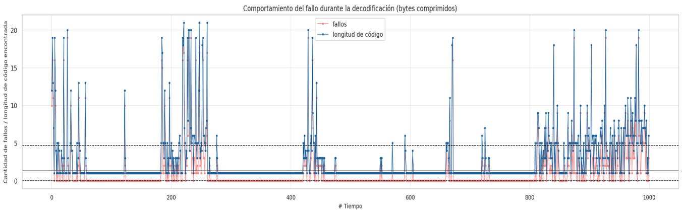
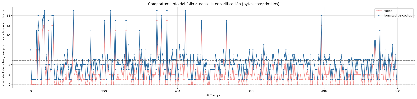
Failure behavior during decoding sorted by compressed bytes
Failure distribution and probability density
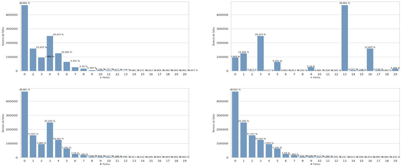
Failure distribution and probability density
Información en el universo holográfico.txt
Failure behavior during decoding using a lookup table

Failure behavior during decoding without sorted
Failure behavior during decoding sorted by lenght codes
Failure behavior during decoding sorted by compressed bytes

Failure distribution and probability density

Failure distribution and probability density
short-text.txt

Failure behavior during decoding using a lookup table
Failure behavior during decoding without sorted
Failure behavior during decoding sorted by lenght codes
Failure behavior during decoding sorted by compressed bytes
Failure distribution and probability density

Failure distribution and probability density
Conclusions
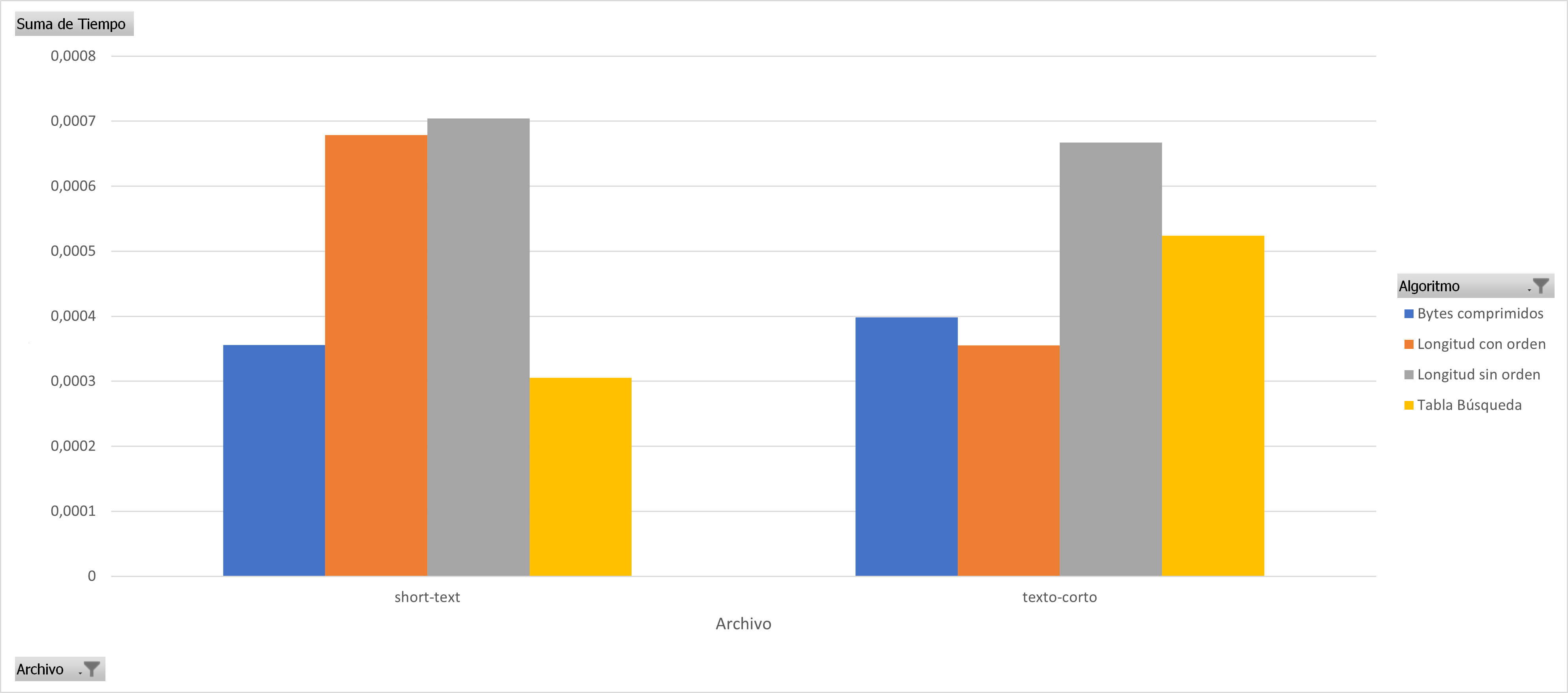
In almost all cases it can be seen that sorting the huffman table by the code lengths containing the most compressed bytes is a better sequential decoding option based on code lengths. The following graphs show the results for each group of files with similar sizes, the decision to separate the graphs into different groups was to keep the Y axis in the same bounds, the decoding technique based on Markov chains was removed since it presents the worst times of decoding in all cases.

Code
You can see the code of the whole project here: Code
Contributing and Feedback
Any ideas or feedback about this repository?. Help me to improve it.
Authors
- Created by Ramses Alexander Coraspe Valdez
- Created on 2020
References
Below we mention some studies performed based on the decompression of huffman codes:
- Balancing decoding speed and memory usage for Huffman codes using quaternary tree (Habib y Rahman, 2017)
- Data-Parallel Finite-State Machines (Mytkowicz, Musuvathi y Schulte, 2014)
- Massively Parallel Huffman Decoding on GPUs (Weißenberger y Schmidt, 2018)
- P-Codec: Parallel Compressed File Decompression Algorithm for Hadoop (Hanafi, I., & Abdel-raouf, A. (2016))